Creating and Using Excel Templates

As an Advanced Excel User, you want to avail yourself of every accessible efficiency tool. Excel Templates are files containing common data and formatting options used as Models for other spreadsheets.

A Template is a great shortcut for standardizing the look and functionality of your data. Templates can also provide you with a Standard Framework in which to input and share your data. Reusable formulas and fields enable you to Speed Up your input and get the information that you want in the form you want.

Creating a Template:

1. Open a worksheet you want to use as the basis for the template
2. Choose Save As and enter a name for the template
3. From the Save as Type list, select Template
4. Save the file inside the Templates folder

Using a Template

1. Go to the File menu and choose New
2. Click on Templates and select the general category
3. Double-click on the desired template
4. A new worksheet opens and displays the template
5. Be sure to Name the worksheet when you save it

That’s all there is to it! Try it out – Templates can Save You a Lot of Work, and help you maintain a consistent, Professional Look.

The Power of Solver!

Microsoft Solver is one of the most Overlooked tools in Excel, and bears occasional review. . As an Excel Guru, it deserves to be part of your repertoire. Although you may not have an immediate need for it, knowing that it exists, and how this Free Add-in works, can result in a future Brainstorm!

"Solver" is an example of how computing power can save you from a plethora of second-guessing. Let's take a look at what it can do and how you can leverage this Powerful Analytic Tool:

Where is it?

To find it in Excel 2010, click on the File Tab, and click the Excel Options button at the bottom of the dropdown. Then choose Add-Ins and select Solver Add-in.

To find it in Excel 2007, simply click on the Microsoft Button, and click the Excel Options button at the bottom of the dropdown. Then choose Add-Ins and select Solver Add-in.

After you load the Solver add-in, the Solver command is available in the Analysis group on the Data tab.

What it can Do for You!

My Classic Example is one where you have several shifts of call center employees that overlap, and you are trying to optimize the scheduling to best handle the projected incoming calls. By using MS Solver, you can quite quickly find the most Favorable Balance for the schedule.

The trick is set your Target Cell (this may be a cell in which you are trying to find the Best Sum, Average, or Standard Deviation) in the Solver Parameters, and make it subject to various cells that you wish to change (in this case, it would be the totals for each shift). You can also make it subject to Constraints such as Whole numbers (good when counting people...).

MS Solver can be effectively used to maximize Sales/Profit Plans, Strategic Planning, Optimizing a Product Mix, and even picking a Winning Team! There are Countless Applications that are only limited by your imagination.

It can take a bit of effort setting up your worksheet, but the results are Outstanding! Demonstrate once again that you truly are a Genius! Give Microsoft Solver a try!

Match plus Index = Power!

You are an Excel Poweruser, and you say you often use the VLOOKUP function, but would like something a bit more versatile and powerful? Look no further than the MATCH and INDEX functions!

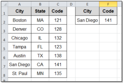
If you want something more versatile than VLOOKUP, MATCH and INDEX can serve as your humble servants. Let’s take a look at a simple example using the Illustration above:

For instance, MATCH returns the Row Number of the location in an array of value you specify. Using the example above, the number “4” is returned by the formula:

=MATCH("Tampa", $A$2:$A$8,0)

INDEX, on the other hand, returns the Value that you identify by row number in an array. Using the example above, “Tampa” is retuned by the formula:

=INDEX($A$2:$A$6,4)

Combining the INDEX and MATCH functions is where the Real Power comes in. Let’s say we want the Code for San Diego. We can set up a Code Retriever as shown in cells E1:F2, by inserting the following formula in cell F2 (This will return "141"):

=INDEX($C$2:$C$8, MATCH(E2, $A$2:$A$8, 0))

Once you try this, you will be Amazed! Using MATCH and INDEX functions together, now that’s POWER!

Options!

In the old Clint Eastwood movie, Magnum Force, Harry Callahan used the line, “A man’s got to know his limitations”. True as that is, Harry always liked to have Options. For this first post of 2012, I thought it would be interesting to take a look at Option Buttons.

Option Buttons can be very useful in creating Quizzes or Polls in Excel, and are not too difficult to create. There are a few steps, but I guarantee that it will be worth the effort! Here is how you do it:

1. Make sure the Developer tab is visible on your toolbar

2. Under the Developer tab, choose Insert / Option Button (Form Control)

3. Draw the Option Button box on your worksheet and repeat for however many buttons you wish to have for choices

4. Now, (this is Important), to make the buttons work together, return to your Insert dropdown and choose Group Box (Form Control)

5. Then draw your Group Box all the way around your Option Buttons

Hooray, We’re Almost There!

6. Right-Click one of the Option Buttons, choose Format Control from the dropdown and select a Cell Link that you want your Option Buttons to populate

7. Now is where the Fun really begins. Create a Formula that is based on the value that is shown in the Cell Link

8. For example, let’s say you have linked three Option Buttons to cell $E$5 and you wanted Option 2 to return a “Correct” response and the others to return “Incorrect”, here is what you do:

In cell E6, type =IF(E5=0,"", IF(E5=3, "Correct!", "Incorrect"))

Now when the user chooses Option 2 of the three possible, they are rewarded with the “Correct” feedback. Option Buttons, give them a try; “It is Always Good to have Options…”

Happy New Year All!

DATEVALUE Function Rules!

A Date is a Date is a Date (well, that certainly wasn’t true back in my college days). Nor is it true in Excel. As an Advanced User, you know that what may look like a Date, may not “play nice” with other dates that you have in your worksheet.

Let’s say that you have inherited an Excel workbook made by some Genius, (please note the thinly veiled sarcasm), and you want to Perform Some Analysis (in your case, truly genius work) that save the company countless hours and expense. The trouble is that unless you can Rely on the consistency of the way Excel will be handling the “Dates” in the worksheets, you Cannot Rely on the efficacy of your results (the old “Garbage In, Garbage Out” cliché).

So what is an Excel Guru like you to do? DATEVALUE to the Rescue! Yes, indeed, my friends, DATEVALUE will calm your nerves, relieve your upset stomach, cure that nagging doubt that you are being watched, and make any Dates in your worksheet work in consistency with all of the dates therein. (Well, I may have exaggerated some of the attributes, but it will make your dates play nice with each other…).DATEVALUE will instantly convert any looks-like-a-date Date into the standard Excel serial number, and you can then format it as you wish.

How Cool is that! It may sound minor matter, but it can save you a world of grief in many circumstances.

Note of Caution: For you Apple Users out there, (I use Excel on a MacBook occasionally myself), Microsoft Excel for the Macintosh uses a different date system as its default (go figure…).

The DATEVALUE function: Good Stuff!

You Want to Ask, “What If?”

"What If” scenarios are a valuable instrument for nearly any business. Any advanced user should be aware that Excel provides a great tool to accomplish this. Excel can automatically make changes in a variable using Goal Seek (it can save you a ton of work, and make you look like a Genius in the process).

Using a very Simple Example, let’s say that you are a call center sales manager, and you know the approximate number of calls you are going to receive for the next month, as well as the sales goal that has been set by the executive branch. You wish to know the Call-To-Sale-Conversion-Rate so you can advise your staff. A rudimentary calculator can be created in the cells of your Excel worksheet as follows:

Number of Calls x Conversion Rate = Number of Sales (e.g. C4*C5 = C6)

After filling in the values for C4 and C6, you can use Goal Seek to calculate the required value for C5.

Obviously, this tool can be used to greater Advantage with more complex scenarios, but you get the picture. Goal Seek can be a handy tool for the boardroom or any planning venue. As am Advanced User, you owe it to yourself to Give it a Try!

Using the Data Entry Form

Since you are an Advanced Excel User, you may have someone other than yourself who frequently adds records to databases or tables that you have created. If this is the case, you should definitely encourage the use of the Data Form Tool. For anyone who routinely enters data, it can make Life a Bit Easier.

How to Add the Form to Your Workbook for Excel 2007 & 2010 Users:

1. Click the down-arrow of the Quick Access Toolbar in the upper-left corner of your workbook

2. Choose Customize Quick Access Toolbar

3. Select All Commands and choose Form…

4. Click the Add>> button and click OK

Now go to your database or table and select the Form from your Quick Access Toolbar. Presto, there is is! Up pops a New Data Entry Form for updating your database!

Just tab through the Form as you enter your data, and watch your table or database update as you do. Wow, what a Great Little Tool! Give it a try!